- 1.Introduction
- 2.Model Tree
- 3.Method demonstration — Boston Housing Price
- 4.Some notice using M5’ Algorithm
- references
Nanjin Zeng(id:15220162202482) WISE IUEC 2016
You can also get a .lyn version in the same github folder because it is written with latex.
1.Introduction
In the challenge “trees”, we are required to find a method to construct a piecewise linear decision tree. It means that we should find a tree-based model, but imposing a linear relationship instead of values on the leaf. In this blog, I want to introduce a method called M5’ Algorithm, which is a common method for buliding Piecewise Linear Decision Tree, or Model Tree. In section 2, I would give a brief explaination for its mechanism and development path. In section 3, I would demonstrate this method using the demo example in lecture, data boston housing price, with a compare with other methods introduced in class.
2.Model Tree
After looking up the journal data base, I find that many algorithms were raised in 1990s might help us to construct this kind of models, like MARS using recursive patitioning to choose the knots[1] (Friedman, 1991/Actually, it is not a tree base model.), SUPPORT (“Smoothed and Unsmoothed Piecewise-Polynomial Regression Trees”, Chaudhuri et al, 1994) selecting its splits by analysis of the distributions of the residuals[2]. But I want to introduce a most popular one, M5 model tree. It is widely used even in other science filed, such as precticting wave height (A Etemad-Shahidi et al, 2009) and river flow forecasting (MT Sattari et al, 2013).
2.1 M5 Algorithm (Quinlan, 1992)
After the invention of CART system for decision trees(Breiman et al, 1984), people were curious about if they could extend this techniques to deal with numerically-valued attributes by choosing a threshold at each node of the tree and testing the value against threshold.[3] But they do not think about the situations that where the class value is numeric. In 1992, an algorithm called M5 was raised by Quinlan, which is a resemble method combining the linear regression function and decision trees.
The procedures buliding a model tree is similar to build a decision tree using CART
- In the first stage, a decision tree induction algorithm is used to bulid a tree. The splitting criterion is based on the standard deviation of the class value. Slighly different to the CART, it does not choose the one gives the greatest expected reduction in variance. It tests it splits by maximizing the standard deviation reduction (SDR), calculated by
\[SDR=sd(T)-\sum_{i}\frac{\left[T_{i}\right]}{\left[T\right]}*sd\left(T_{i}\right)\]
where \(T\) is the set of examples that reach the node and \(T_{i}\) is the set that result from splitting the node accordiung to the chosen attribute.
-
After buliding the initial tree, the second stage is to prune the tree. First, the absolute error is averaged for each of the training examples that reach that node. To compensate the underestimate of the \(E_{out}\), it is multiplied by the factor \(\frac{n+v}{n-v}\) ,where n is the number of training example that reach the node and v is the number of training examples that reach the node and v is the number of parameters in the model. To notice, the model is calculated using only the attributes that are tested in the subtree below this node. That could be a fair compare with subtree. Once a linear model constructed in this way is in place for a interior node, the tree is pruned back from the leaves.
- The final stage is a smoothing process. It is a complex process so I want to skip it. But the basic idea is that, this process decrease the discountinuitics between adjacent linear models at the leaves, which is believed to increase the accuracy of preductions.
The author claims and illustrates it with data that this M5 model tree have advantages over regression trees in both compactness and predition accuracy, attributable to the abiliy of model trees to exploit local linearity in data.
2.2 M5’ Algorithm (Wang & Witten, 1997)
As a resemble method combining linear regression and decision trees, the M5 model tree give high prediction accuracy with the small price on interpretation. But for the prototype in 1992, it still has some ambigious point.
-
It do not allow a split that create a leaf with fewer than two training examples. \((n=v=1)\)
-
M5 do not split a node if it represents very few examples or their values vary only slightly. The author shows that the result are not very sensitive to the choice of threshold.[3]
-
At the pruning process, attributes are dropped from a model when their effect is somall. But this criterion is too strict, sometimes these attributes may participate in higher level model.
-
M5 do not give a clear notice how to deal with missing attribute values.
In order to ease these draw back, they give a improved algorithm called M5’. Being brief, I focus on the main improvement of this model. It modified the SDR to
\[SDR=\frac{M}{\left[T\right]}*\beta\left(i\right)*\left[sd(T)-\sum_{j\in\left\{ I,R\right\} }\frac{\left[T_{j}\right]}{\left[T\right]}*sd\left(T_{j}\right)\right]\]\(m\) is the number of examples without missing values for that attribute. \(\beta\left(i\right)\) is the correction factor which is unity for a binary split and decays exponentially as the number of values increases.
The author states, they first deal with all examples for which the value of the spliting attribute is known. If it is continous, they determine a numeric threshold for splitting in the usual way. For each split point, they calculate the SDR according to this formular.[]
To conclude, this system deals effectively with both enumcrated attributes and missing attribute values. It has the advantage that the models it generates are compact and relatively comprehensible.
3.Method demonstration — Boston Housing Price
In application, we could use a R pack called “Rweka” to realize M5’ Algorithm. Noticed that it is based on Java, you should have a Java SE environment and R pack “rJava” on your mechine.
The basic syntax is that[4]
M5P(formula, data, subset, na.action, control=weka_control(), options=NULL)
In this case, precluded by the length of this blog, I do not want to introduce advanced option of this function based on Weka algorithm.
First, we create trainning and test sets.
require(MASS)
set.seed(1234) #set random seed in order to repeat the result
train = sample(nrow(Boston), nrow(Boston)*0.6)
data_train = Boston[train,]
data_test = Boston[-train,]
For the main part,
require(RWeka)
m.m5p <- M5P(medv~.,data=data_train) #train the classifier using training data
yhat <- predict(m.m5p,data_test) #test the classifier using L2 loss
mean((yhat-ytrue)^2)
Here is the error on the test data, comparing to other algorithm we have learnt in class.
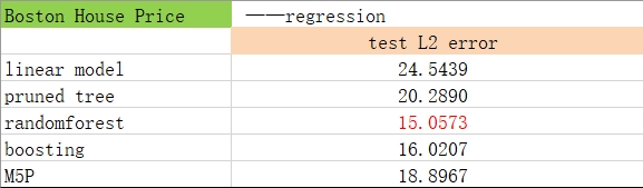
The random forest is still the best. As a resemble method, M5P beats pruned decision tree and linear model in prediction accuracy, in a price of being less interpretable. The test result is consistant as we expected.
4.Some notice using M5’ Algorithm
From the discussion and example above, we can clearly know some features of M5’ algorithm.
-
As a resemble method, M5’ Algortithm fits linear regression model instead a constant in leaves. It enhances the prediction accuracy, in a price of being less interpretable. We should make a trade-off if we are doing a research, since we sometimes need to reveal the pattern underlying the sample to make some intrepretations, more than making good predictions on data. We could not apply it blindly because it seems more accurate.
-
For other simulation data in lecture, their class value is binary. In this case, we could not use M5P algorithm. Obviously, in this case, fitting a linear relationship on the leaves do not make sense. In applications, researchers using this algorithm mainly in something may have a numerical outcome, like water level and the melt tempreture on alloy. Actually, the M5P algorithm do not run if it detects that you outcome is binary.
references
[1] Friedman, Jerome H. “Multivariate Adaptive Regression Splines.”[J], The Annals of Statistics 19, no. 1 (1991): 1-67. http://www.jstor.org/stable/2241837.
[2]Chaudhuri, Probal, Min-Ching Huang, Wei-Yin Loh, and Ruji Yao. “PIECEWISE-POLYNOMIAL REGRESSION TREES.”[J], Statistica Sinica 4, no. 1 (1994): 143-67. http://www.jstor.org/stable/24305278.
[3]Wang, Y. & Witten, I. H. (1996). Induction of model trees for predicting continuous classes. (Working paper 96/23)[R]. Hamilton, New Zealand: University of Waikato, Department of Computer Science.
[4]K. Hornik, C. Buchta, and A. Zeileis. Open-source machine learning: R meets Weka.[J] Computational Statistics, 24(2):225{232, 2009. doi: 10.1007/s00180-008-0119-7.
[5]JR Quinlan. Learning with continuous classes[A]. Anthony Adams and Leon Sterling. AI ‘92[C]. Proceedings of the 5th Australian Joint Conference on Artificial Intelligence. (1992). doi:10.1142/9789814536271
[6]Jiaming Mao. “Decision_Trees_and_Ensemble_Methods”[Z].2019-05-05.personal copy