- 1.Introduction
- 2.Back to the origin
- 3 An Example Using Stata 15.0
- 4 Why we choose to use Bootstrap Method?
- references
Nanjin Zeng(id:15220162202482) WISE IUEC 2016
Bug fixed! You need not wait for mathemetical formulas to load.
You can also get a .lyn version in the same github folder because it is written with latex.
1.Introduction
In the lecture, we have learnt an amazing method, bootstrap, which processes sounds very easy
The bootstrap approach generates new samples by repeatedly drawing observations from the observed sample with replacement, which could be used to quantify the uncertainty accociate with a given estimator or statistical menthod.
I wonder how this method works well and what the advantage of this method is. In the following part, I would introduce the idea behind this method first. Then I will show how to run this method using Stata15.
2.Back to the origin
2.1 Jackknife method
After reading the paper of Efron(1979), the first paper carry out this idea, I know more about this method. Before Efron raised this method, the statisticians used another diffenent resampling method, Jackknife method by Quenouille(1956). The process of this method is also insteresting.
Let \(T_{n}=T(X_{1},\cdots,X_{n})\) be a statistic and \(T_{(-i)}\) denote the statistice with the \(i^{th}\) observation removed. Let \(\overline{T_{n}}=\frac{\sum_{i=1}^{n}T_{(-i)}}{n}\). The jackknife estimate of \(Var(T_{n})\)is[2]
\[v_{jack}=\frac{n-1}{n}\sum_{i=1}^{n}(T_{(-i)}-\overline{T_{n}})^{2}\]
It means that we take one of the observations for sample each time. Then we get n jackknife samples. Then we use these samples to recompute the estimator.
2.2 Bootstrap method
And for the bootstrap method, the process is stated in the lecture. After reading the paper, being precisely, it could be divided into two process.
Construct the sample probability distribution \(\hat{F}\), putting mass 1/n at each point \(x_{1},x_{2},\cdots,x_{n}\).
With \(\hat{F}\)fixed, draw a random sample of size n from \(\hat{F}\). Approximatemate the sampling distribution of estimator(random variable) by the bootstrap distribution.[3]
Further more, for step 2, three methods are given by the author. To some estimator like sample mean, we can write down a simple formula for variance (method 1). We can also use Tarlor series expansion (method 3). But the common way we use these days is Monte Carlo approximation (method 2). Repeated realizations of \(X^{*}\) are generated by taking random samples of size \(n\) from \(F\), which is a way as simulation.
By these process, we use two approximations. In step 1, we use an construsted empricial distribution \(\hat{F}\) to approximate the true \(F\). In step 2, we use the variance of the estimator in these bootstrap samples to estimates the variance. The uncertainty of this processmainly comes form first approximation, because we can make \(B\rightarrow\infty\). It also state that though it could work well with uncertain distribution and small sample, it could not save you from a totally “bad” samples, like one just have two observations. In this case, you could not expect that your constructed EDF could be compatible with the true CDF.[2]
\[v_{boot}=\frac{1}{B}(\sum_{r=1}^{B}T_{n,b}^{*}-\frac{1}{B}\sum_{r=1}^{B}T_{n,r}^{*})^{2}\]
Comparing with Jackknife method, it has some improvements. First, it is more general, for example, the jackknife estimate do not work well with the stand error of sample quantiles[4]. Second, at Quenouille’s time, they do not have computer to draw random sample and compute the estimator each by each for so many bootstrap samples. But we could run bootstrap using statistic programmes. We could enlarge the resampling by taking more than 1000 bootstrap samples. That means it is out performed by the bootstrap when \(B\rightarrow\infty\).
3 An Example Using Stata 15.0
As I mentioned above, thanks to the development of computer science. We could use bootstrap method costlessly. In this part, I will show how to run bootstrap method using a group of simulated data.
Let’s use the same example as the lectnotes in OLS. First we genenrate a data with only 20 observations.
set obs 20
gen x1 = uniform()
gen x2 = 0.5x1 + 0.5rnormal(0,1)
gen e = rnormal(0,1)
gen y = 1 - 2.5x1 + 5x2 + e
To use bootstrap, we need the command bootstrap, the syntax is[5]
bootstrap exp list [, options] : command
To simple use, we could determin the number of samples with reps(#), which default is 50, but to rules of thumb it should be more than 1000. And we could save the results by attaching _b,saving(bstat). More options are available looking up the help file. command is any command follows standard Stata syntax. In this case we use
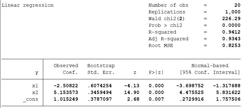
bootstrap _b, saving(bstat) reps(1000) bca:reg y x1 x2,r

The bootstrap standard error is stated at the second row.
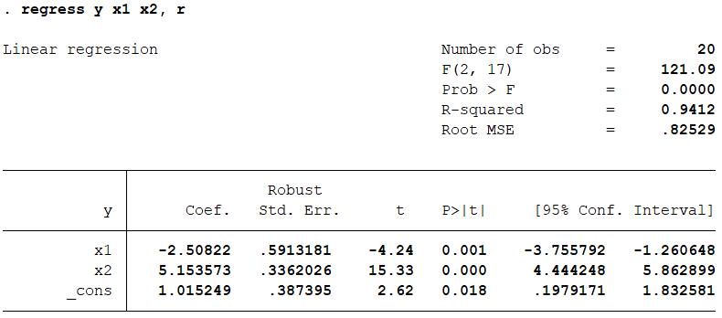
Let compare it to the robust standard error if we run the regression directly.

The error only slightly differs to each other! It reveals that if \(B\rightarrow\infty\), Monte Carlo approximation (method 2) could behave nearly as well as using formula for variance in specific distribution (method 1).
4 Why we choose to use Bootstrap Method?
From the example, we can clearly know the advantage using bootstrap method.
- You do not need to worry about how to derive the varicance formula of your estimator. All you have to do is to simulate it using you computer. It could be very useful when you have an unusual or complex estimator, like what we talked in the lecture, the \(\hat{\alpha}\) for the total risk in two fianancial assets.
- As a nonparametric method, your could use it regardless much prior assumptions. It only needs some simple assumpions like i.i.d samples. As the example above, though the \(se()\) is derived from Heteroskedasticity Robust Standard Error formula, it is based on the three OLS assumptions. If some of them are violated, the estimation is unreliable. However, bootstrap \(se()\) is still reliable in this case. (But you should not continue use OLS coefficient estimator without these assumption.XD)
- Bootstrap method have much more applications than finding variances for estimator. For example, it can reveal the bias of estimator in that case. It could also be used in hypothesuis and specification test, empiricial likelihood in overidentified mofel, …[4]
references
[1] Jiaming Mao. “Regression”[Z].2019-03-30.https://github.com/jiamingmao/data-analysis/blob/master/Lectures/Regression.pdf
[2]AC Cameron, PK Trivedi. “Microeconometrics”[M].Cambridge Books.2008.107-118
[3]Efron, B. “Bootstrap Methods: Another Look at the Jackknife.”[J].The Annals of Statistics 7, no. 1 (1979): 1-26
[4]Larry Wasserman. “All of Statistics: A Concise Course in Statistical Inference”[M].Springer Science & Business Media.2013.357-383
[5]Stata Statistics/Data Analysis. “bootstrap_bootstrap sampling and estimation”[Z]. 2019-03-30.
[6]Efron, B., and R. Tibshirani. “Bootstrap Methods for Standard Errors, Confidence Intervals, and Other Measures of Statistical Accuracy.”[J].Statistical Science 1, no. 1 (1986): 54-75.
Weekly Recommended Reading by myself
Contributors receive social benefits from their contributions, and the shrinking group size reduces these social benefits.
JOURNAL ARTICLE
Group Size and Incentives to Contribute: A Natural Experiment at Chinese Wikipedia
Xiaoquan (Michael) Zhang and Feng Zhu
The American Economic Review Vol. 101, No. 4 (JUNE 2011), pp. 1601-1615 (15 pages) Published by: American Economic Association
DOI: 10.1257/aer.101.4.1601
As our previous learning in priciple class, the content in Wiki is a kind of public goods. It means that the contributors could not charge fee for their contribution. That comes the free rider problem. Moreover, as the size of users grows, the users would be more unwilling to contribute because he could expect others to do it for him. But the author evaluates the effect of the block by mainland and find that the result is in opposite. That is a very unexpected idea. Furthermore, the methodology they used is not so complex. You could spend some fragmented time to read it even the midterm is coming.
